Reproducing plots of the illustrative example of the paper¶

Code for reproducing the plots related to the illustrative example presented in the paper

import numpy as np
import mne
import os.path as op
import os
import pooch
import matplotlib.pyplot as plt
import math
import funcs_single_sim as funcs
from mpl_toolkits.axes_grid1 import make_axes_locatable
target = '..'


def crop_image(image_matrix):
    image = image_matrix.copy()
    i_left = 0
    i_right = image.shape[1] - 1
    i_top = 0
    i_bottom = image.shape[0] - 1
    while np.array_equal(image[:, i_left, :], image[:, 0, :]):
        i_left += 1

    while np.array_equal(image[:, i_right, :], image[:, -1, :]):
        i_right -= 1

    while np.array_equal(image[i_top, :, :], image[0, :, :]):
        i_top += 1

    while np.array_equal(image[i_bottom, :, :], image[-1, :, :]):
        i_bottom -= 1

    cropped_image = image_matrix[i_top -
                                 10:i_bottom + 10, i_left - 10:i_right + 10]
    return cropped_image

Download data (if not already downloaded or generated with generate_fwd.py)

data_path = op.join('..', 'data')
data_single_sim_path = op.join('..', 'data', 'data_single_sim')

if not op.exists(data_path):
    os.mkdir(data_path)

if not op.exists(data_single_sim_path):
    os.mkdir(data_single_sim_path)

fname = 'connectivity.npy'
if not op.exists(op.join(data_single_sim_path, fname)):
    url = 'https://osf.io/download/zfwxh/?direct%26mode=render'
    pooch.retrieve(url=url, known_hash=None,
                   path=data_single_sim_path, fname=fname)

fname = 'data.npy'
if not op.exists(op.join(data_single_sim_path, fname)):
    url = 'https://osf.io/download/a8xdn/?direct%26mode=render'
    pooch.retrieve(url=url, known_hash=None,
                   path=data_single_sim_path, fname=fname)

fname = 'features.npy'
if not op.exists(op.join(data_single_sim_path, fname)):
    url = 'https://osf.io/download/kzxad/?direct%26mode=render'
    pooch.retrieve(url=url, known_hash=None,
                   path=data_single_sim_path, fname=fname)

fname = 'parameters.npy'
if not op.exists(op.join(data_single_sim_path, fname)):
    url = 'https://osf.io/download/zcsgv/?direct%26mode=render'
    pooch.retrieve(url=url, known_hash=None,
                   path=data_single_sim_path, fname=fname)


fname = 'oct6_fwd.fif'
if not op.exists(op.join(data_path, fname)):
    url = 'https://osf.io/download/7dfvm/?direct%26mode=render'
    pooch.retrieve(url=url, known_hash=None, path=data_path, fname=fname)

fname = 'cortico_dist_oct6.npy'
if not op.exists(op.join(data_path, fname)):
    url = 'https://osf.io/download/37kaz/?direct%26mode=render'
    pooch.retrieve(url=url, known_hash=None, path=data_path, fname=fname)

Load data

connectivity_file = op.join(data_single_sim_path, 'connectivity.npy')
connectivity = np.load(connectivity_file, allow_pickle=True).item()

data_file = op.join(data_single_sim_path, 'data.npy')
data = np.load(data_file, allow_pickle=True).item()

features_file = op.join(data_single_sim_path, 'features.npy')
features = np.load(features_file, allow_pickle=True).item()

parameters_file = op.join(data_single_sim_path, 'parameters.npy')
parameters = np.load(parameters_file, allow_pickle=True).item()

fwd_file = op.join(data_path, 'oct6_fwd.fif')
fwd = mne.read_forward_solution(fwd_file, verbose=False)
fwd = mne.convert_forward_solution(fwd, surf_ori=True, force_fixed=True,
                                   use_cps=True, verbose=False)
fwd = mne.pick_types_forward(fwd, meg='mag', eeg=False, ref_meg=False)

cortico_dist_file = op.join(target, 'data', 'cortico_dist_oct6.npy')
cortico_dist = np.load(cortico_dist_file)

102 out of 306 channels remain after picking

Define additional features

G = fwd['sol']['data']  # leadfield matrix
G = 10**5*G
GGt = G.dot(G.T)
U, s, V = np.linalg.svd(G)
V = V.T

dip_pos = fwd['source_rr']
dip_or = fwd['source_nn']
src = fwd['src']
vertno = [src[0]['vertno'], src[1]['vertno']]

X = data['X']
Y = data['Y']
seed_loc = data['sees_loc']
lamX = parameters['tc']
AUC_conn = parameters['conn']
TPF_conn = parameters['TPF_conn']
FPF_conn = parameters['FPF_conn']
area = features['area']
r = np.sqrt(area*10**(-4)/math.pi)
p1_locs, p2_locs = funcs.gen_patches_sources(cortico_dist, r, seed_loc)
lambdas = np.logspace(-5, 1, num=15)
M = G.shape[0]
N_dense = G.shape[1]
fs = features['fs']
nperseg = 256
nfft = nperseg
fmin = features['fmin']
fmax = features['fmax']

Optimal parameters

lam_cps = lambdas[np.argmin(AUC_conn[0, :])]*lamX
lam_imcoh = lambdas[np.argmin(AUC_conn[1, :])]*lamX
lam_ciplv = lambdas[np.argmin(AUC_conn[2, :])]*lamX
lam_wpli = lambdas[np.argmin(AUC_conn[3, :])]*lamX

lam_cps = lambdas[np.argmin(AUC_conn[0, :])]*lamX
lam_imcoh = lambdas[np.argmin(AUC_conn[1, :])]*lamX
lam_ciplv = lambdas[np.argmin(AUC_conn[2, :])]*lamX
lam_wpli = lambdas[np.argmin(AUC_conn[3, :])]*lamX

Estimated neural activity with the optimal parameters

X_lamX = ((G.T).dot(np.linalg.inv(G.dot(G.T)+lamX*np.eye(M)))).dot(Y)
X_lam_cps = ((G.T).dot(np.linalg.inv(G.dot(G.T)+lam_cps*np.eye(M)))).dot(Y)
X_lam_imcoh = ((G.T).dot(np.linalg.inv(G.dot(G.T)+lam_imcoh*np.eye(M)))).dot(Y)
X_lam_ciplv = ((G.T).dot(np.linalg.inv(G.dot(G.T)+lam_ciplv*np.eye(M)))).dot(Y)
X_lam_wpli = ((G.T).dot(np.linalg.inv(G.dot(G.T)+lam_wpli*np.eye(M)))).dot(Y)

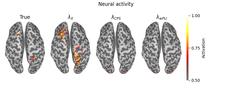
Plot neural activity

hemi = 'both'
subject_dir = op.join(mne.datasets.sample.data_path(), 'subjects')
subject = 'sample'

clim = {'kind': 'value', 'lims': [0.5, 0.75, 1]}
roll = 0

views = 'axial'
size = (1200, 1000)

# plot simulated seed based connectivity
stc = mne.SourceEstimate(np.linalg.norm(X, axis=1) /
                         np.max(np.linalg.norm(X, axis=1)),
                         vertices=vertno, tmin=0, tstep=1, subject=subject)
brain = stc.plot(subject=subject, surface='inflated', smoothing_steps=5,
                 views=views, size=size, clim=clim, hemi=hemi,
                 subjects_dir=subject_dir, time_viewer=False, colorbar=False,
                 background='white', add_data_kwargs=dict(
                     colorbar_kwargs=dict(label_font_size=40)))
brain.show_view(azimuth=-90, elevation=10, distance=600, roll=roll)
screenshot = brain.screenshot()
brain.close()
screenshot1 = crop_image(screenshot)

# plot reconstructed seed brain activity (estimateed using lamX)
stc = mne.SourceEstimate(np.linalg.norm(X_lamX, axis=1) /
                         np.max(np.linalg.norm(X_lamX, axis=1)),
                         vertices=vertno, tmin=0, tstep=1, subject=subject)
brain = stc.plot(subject=subject, surface='inflated', smoothing_steps=5,
                 views=views, size=size, clim=clim, hemi=hemi,
                 subjects_dir=subject_dir, time_viewer=False, colorbar=False,
                 background='white', add_data_kwargs=dict(
                     colorbar_kwargs=dict(label_font_size=40)))
brain.show_view(azimuth=-90, elevation=10, distance=600, roll=roll)
screenshot = brain.screenshot()
brain.close()
screenshot2 = crop_image(screenshot)

# plot reconstructed brain activity (estimateed using lam_cps)
stc = mne.SourceEstimate(np.linalg.norm(X_lam_cps, axis=1) /
                         np.max(np.linalg.norm(X_lam_cps, axis=1)),
                         vertices=vertno, tmin=0, tstep=1, subject=subject)
brain = stc.plot(subject=subject, surface='inflated', smoothing_steps=5,
                 views=views, size=size, clim=clim, hemi=hemi,
                 subjects_dir=subject_dir, time_viewer=False, colorbar=False,
                 background='white', add_data_kwargs=dict(
                     colorbar_kwargs=dict(label_font_size=40)))
brain.show_view(azimuth=-90, elevation=10, distance=600, roll=roll)
screenshot = brain.screenshot()
brain.close()
screenshot3 = crop_image(screenshot)

# plot reconstructed brain activity (estimateed using lam_wpli)
stc = mne.SourceEstimate(np.linalg.norm(X_lam_wpli, axis=1) /
                         np.max(np.linalg.norm(X_lam_wpli, axis=1)),
                         vertices=vertno, tmin=0, tstep=1, subject=subject)
brain = stc.plot(subject=subject, surface='inflated', smoothing_steps=5,
                 views=views, size=size, clim=clim, hemi=hemi,
                 subjects_dir=subject_dir, time_viewer=False, colorbar=False,
                 background='white', add_data_kwargs=dict(
                     colorbar_kwargs=dict(label_font_size=40)))
brain.show_view(azimuth=-90, elevation=10, distance=600, roll=roll)
screenshot = brain.screenshot()
brain.close()
screenshot4 = crop_image(screenshot)

fig, ax = plt.subplots(1, 5, figsize=(8, 3))
ax[0].imshow(screenshot1)
ax[0].axis('off')
ax[0].set_title('True')

ax[1].imshow(screenshot2)
ax[1].axis('off')
ax[1].set_title(r'$\lambda_{{X}}$')

ax[2].imshow(screenshot3)
ax[2].axis('off')
ax[2].set_title(r'$\lambda_{{CPS}}$')

ax[3].imshow(screenshot4)
ax[3].axis('off')
ax[3].set_title(r'$\lambda_{{wPLI}}$')

ax[4].axis('off')
divider = make_axes_locatable(ax[4])
cax = divider.append_axes('left', size='5%', pad='0%')
cbar = mne.viz.plot_brain_colorbar(cax, clim, 'hot', bgcolor='0.5')

fig.suptitle('Neural activity')
plt.tight_layout()

$Neural activity, True, $\lambda_{{X}}$, $\lambda_{{CPS}}$, $\lambda_{{wPLI}}$$

Using pyvistaqt 3d backend.

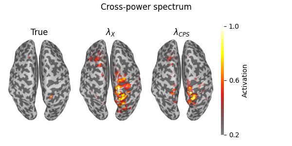
Plot cross-power spectrum

cps_true = connectivity['conn_true'][:, :, 0]
cps_lam_cps = connectivity['conn_lamC'][:, :, 0]
cps_lamX = connectivity['conn_lamX'][:, :, 0]

clim = {'kind': 'value', 'lims': [0.20, 0.6, 1]}

# Plot true cross-power spectrum
stc = mne.SourceEstimate(np.mean(cps_true, axis=0) /
                         np.max(np.mean(cps_true, axis=0)), vertices=vertno,
                         tmin=0, tstep=1, subject=subject)
brain = stc.plot(subject=subject, surface='inflated', smoothing_steps=5,
                 clim=clim, views=views, size=size, hemi=hemi,
                 subjects_dir=subject_dir, time_viewer=False, colorbar=False,
                 background='white', add_data_kwargs=dict(
                     colorbar_kwargs=dict(label_font_size=40)))
brain.show_view(azimuth=-90, elevation=10, distance=600, roll=roll)
screenshot = brain.screenshot()
brain.close()
screenshot1 = crop_image(screenshot)


# Plot estimated cross-power spectrum (using lamX)
stc = mne.SourceEstimate(np.mean(cps_lamX, axis=0) /
                         np.max(np.mean(cps_lamX, axis=0)), vertices=vertno,
                         tmin=0, tstep=1, subject=subject)
brain = stc.plot(subject=subject, surface='inflated', smoothing_steps=5,
                 clim=clim, views=views, size=size, hemi=hemi,
                 subjects_dir=subject_dir, time_viewer=False, colorbar=False,
                 background='white', add_data_kwargs=dict(
                     colorbar_kwargs=dict(label_font_size=40)))
brain.show_view(azimuth=-90, elevation=10, distance=600, roll=roll)
screenshot = brain.screenshot()
brain.close()
screenshot2 = crop_image(screenshot)

# Plot estimated cross-power spectrum (using lam_cps)
stc = mne.SourceEstimate(np.mean(cps_lam_cps, axis=0) /
                         np.max(np.mean(cps_lam_cps, axis=0)), vertices=vertno,
                         tmin=0, tstep=1, subject=subject)
brain = stc.plot(subject=subject, surface='inflated', smoothing_steps=5,
                 clim=clim, views=views, size=size, hemi=hemi,
                 subjects_dir=subject_dir, time_viewer=False, colorbar=False,
                 background='white', add_data_kwargs=dict(
                     colorbar_kwargs=dict(label_font_size=40)))
brain.show_view(azimuth=-90, elevation=10, distance=600, roll=roll)
screenshot = brain.screenshot()
brain.close()
screenshot3 = crop_image(screenshot)

fig, ax = plt.subplots(1, 4, figsize=(6, 3))
ax[0].imshow(screenshot1)
ax[0].axis('off')
ax[0].set_title('True')

ax[1].imshow(screenshot2)
ax[1].axis('off')
ax[1].set_title(r'$\lambda_{{X}}$')

ax[2].imshow(screenshot3)
ax[2].axis('off')
ax[2].set_title(r'$\lambda_{{CPS}}$')

ax[3].axis('off')
divider = make_axes_locatable(ax[3])
cax = divider.append_axes('left', size='5%', pad='0%')
cbar = mne.viz.plot_brain_colorbar(cax, clim, 'hot', bgcolor='0.5')

fig.suptitle('Cross-power spectrum')
plt.tight_layout()

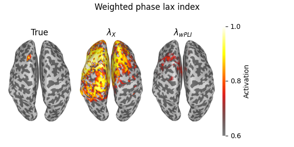
$Cross-power spectrum, True, $\lambda_{{X}}$, $\lambda_{{CPS}}$$

Plot wPLI

wpli_true = connectivity['conn_true'][:, :, 3]
wpli_lam_wpli = connectivity['conn_lamC'][:, :, 3]
wpli_lamX = connectivity['conn_lamX'][:, :, 3]

clim = {'kind': 'value', 'lims': [0.60, 0.8, 1]}

# Plot true wPLI
stc = mne.SourceEstimate(np.mean(wpli_true, axis=0) /
                         np.max(np.mean(wpli_true, axis=0)), vertices=vertno,
                         tmin=0, tstep=1, subject=subject)
brain = stc.plot(subject=subject, surface='inflated', smoothing_steps=5,
                 clim=clim, views=views, size=size, hemi=hemi,
                 subjects_dir=subject_dir, time_viewer=False, colorbar=False,
                 background='white', add_data_kwargs=dict(
                     colorbar_kwargs=dict(label_font_size=40)))
brain.show_view(azimuth=-90, elevation=10, distance=600, roll=roll)
screenshot = brain.screenshot()
brain.close()
screenshot1 = crop_image(screenshot)


# Plot estimated wPLI (using lamX)
stc = mne.SourceEstimate(np.mean(wpli_lamX, axis=0) /
                         np.max(np.mean(wpli_true, axis=0)), vertices=vertno,
                         tmin=0, tstep=1, subject=subject)
brain = stc.plot(subject=subject, surface='inflated', smoothing_steps=5,
                 clim=clim, views=views, size=size, hemi=hemi,
                 subjects_dir=subject_dir, time_viewer=False, colorbar=False,
                 background='white', add_data_kwargs=dict(
                     colorbar_kwargs=dict(label_font_size=40)))
brain.show_view(azimuth=-90, elevation=10, distance=600, roll=roll)
screenshot = brain.screenshot()
brain.close()
screenshot2 = crop_image(screenshot)

# Plot estimated wPLI (using lam_wPLI)
stc = mne.SourceEstimate(np.mean(wpli_lam_wpli, axis=0) /
                         np.max(np.mean(wpli_true, axis=0)), vertices=vertno,
                         tmin=0, tstep=1, subject=subject)
brain = stc.plot(subject=subject, surface='inflated', smoothing_steps=5,
                 clim=clim, views=views, size=size, hemi=hemi,
                 subjects_dir=subject_dir, time_viewer=False, colorbar=False,
                 background='white', add_data_kwargs=dict(
                     colorbar_kwargs=dict(label_font_size=40)))
brain.show_view(azimuth=-90, elevation=10, distance=600, roll=roll)
screenshot = brain.screenshot()
brain.close()
screenshot3 = crop_image(screenshot)

fig, ax = plt.subplots(1, 4, figsize=(6, 3))
ax[0].imshow(screenshot1)
ax[0].axis('off')
ax[0].set_title('True')

ax[1].imshow(screenshot2)
ax[1].axis('off')
ax[1].set_title(r'$\lambda_{{X}}$')

ax[2].imshow(screenshot3)
ax[2].axis('off')
ax[2].set_title(r'$\lambda_{{wPLI}}$')

ax[3].axis('off')
divider = make_axes_locatable(ax[3])
cax = divider.append_axes('left', size='5%', pad='0%')
cbar = mne.viz.plot_brain_colorbar(cax, clim, 'hot', bgcolor='0.5')

fig.suptitle('Weighted phase lax index')
plt.tight_layout()

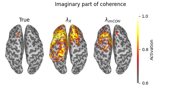
$Weighted phase lax index, True, $\lambda_{{X}}$, $\lambda_{{wPLI}}$$

Plot imCOH

imcoh_true = connectivity['conn_true'][:, :, 1]
imcoh_lam_imcoh = connectivity['conn_lamC'][:, :, 1]
imcoh_lamX = connectivity['conn_lamX'][:, :, 1]

clim = {'kind': 'value', 'lims': [0.60, 0.8, 1]}

# Plot true imCOH
stc = mne.SourceEstimate(np.mean(imcoh_true, axis=0) /
                         np.max(np.mean(imcoh_true, axis=0)), vertices=vertno,
                         tmin=0, tstep=1, subject=subject)
brain = stc.plot(subject=subject, surface='inflated', smoothing_steps=5,
                 clim=clim, views=views, size=size, hemi=hemi,
                 subjects_dir=subject_dir, time_viewer=False, colorbar=False,
                 background='white', add_data_kwargs=dict(
                     colorbar_kwargs=dict(label_font_size=40)))
brain.show_view(azimuth=-90, elevation=10, distance=600, roll=roll)
screenshot = brain.screenshot()
brain.close()
screenshot1 = crop_image(screenshot)


# Plot estimated imCOH (using lamX)
stc = mne.SourceEstimate(np.mean(imcoh_lamX, axis=0) /
                         np.max(np.mean(imcoh_lamX, axis=0)), vertices=vertno,
                         tmin=0, tstep=1, subject=subject)
brain = stc.plot(subject=subject, surface='inflated', smoothing_steps=5,
                 clim=clim, views=views, size=size, hemi=hemi,
                 subjects_dir=subject_dir, time_viewer=False, colorbar=False,
                 background='white', add_data_kwargs=dict(
                     colorbar_kwargs=dict(label_font_size=40)))
brain.show_view(azimuth=-90, elevation=10, distance=600, roll=roll)
screenshot = brain.screenshot()
brain.close()
screenshot2 = crop_image(screenshot)

# Plot estimated imCOH (using lam_imcoh)
stc = mne.SourceEstimate(np.mean(imcoh_lam_imcoh, axis=0) /
                         np.max(np.mean(imcoh_lam_imcoh, axis=0)),
                         vertices=vertno, tmin=0, tstep=1, subject=subject)
brain = stc.plot(subject=subject, surface='inflated', smoothing_steps=5,
                 clim=clim, views=views, size=size, hemi=hemi,
                 subjects_dir=subject_dir, time_viewer=False, colorbar=False,
                 background='white', add_data_kwargs=dict(
                     colorbar_kwargs=dict(label_font_size=40)))
brain.show_view(azimuth=-90, elevation=10, distance=600, roll=roll)
screenshot = brain.screenshot()
brain.close()
screenshot3 = crop_image(screenshot)

fig, ax = plt.subplots(1, 4, figsize=(6, 3))
ax[0].imshow(screenshot1)
ax[0].axis('off')
ax[0].set_title('True')

ax[1].imshow(screenshot2)
ax[1].axis('off')
ax[1].set_title(r'$\lambda_{{X}}$')

ax[2].imshow(screenshot3)
ax[2].axis('off')
ax[2].set_title(r'$\lambda_{{imCOH}}$')

ax[3].axis('off')
divider = make_axes_locatable(ax[3])
cax = divider.append_axes('left', size='5%', pad='0%')
cbar = mne.viz.plot_brain_colorbar(cax, clim, 'hot', bgcolor='0.5')

fig.suptitle('Imaginary part of coherence')
plt.tight_layout()

$Imaginary part of coherence, True, $\lambda_{{X}}$, $\lambda_{{imCOH}}$$

Plot ciPLV

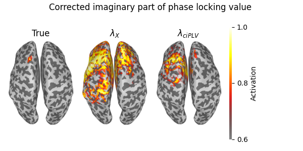
ciplv_true = connectivity['conn_true'][:, :, 1]
ciplv_lam_ciplv = connectivity['conn_lamC'][:, :, 1]
ciplv_lamX = connectivity['conn_lamX'][:, :, 1]

clim = {'kind': 'value', 'lims': [0.60, 0.8, 1]}

# Plot true ciPLV
stc = mne.SourceEstimate(np.mean(ciplv_true, axis=0) /
                         np.max(np.mean(ciplv_true, axis=0)), vertices=vertno,
                         tmin=0, tstep=1, subject=subject)
brain = stc.plot(subject=subject, surface='inflated', smoothing_steps=5,
                 clim=clim, views=views, size=size, hemi=hemi,
                 subjects_dir=subject_dir, time_viewer=False, colorbar=False,
                 background='white', add_data_kwargs=dict(
                     colorbar_kwargs=dict(label_font_size=40)))
brain.show_view(azimuth=-90, elevation=10, distance=600, roll=roll)
screenshot = brain.screenshot()
brain.close()
screenshot1 = crop_image(screenshot)


# Plot estimated ciPLV (using lamX)
stc = mne.SourceEstimate(np.mean(ciplv_lamX, axis=0) /
                         np.max(np.mean(ciplv_lamX, axis=0)), vertices=vertno,
                         tmin=0, tstep=1, subject=subject)
brain = stc.plot(subject=subject, surface='inflated', smoothing_steps=5,
                 clim=clim, views=views, size=size, hemi=hemi,
                 subjects_dir=subject_dir, time_viewer=False, colorbar=False,
                 background='white', add_data_kwargs=dict(
                     colorbar_kwargs=dict(label_font_size=40)))
brain.show_view(azimuth=-90, elevation=10, distance=600, roll=roll)
screenshot = brain.screenshot()
brain.close()
screenshot2 = crop_image(screenshot)

# Plot estimated ciPLV (using lam_ciplv)
stc = mne.SourceEstimate(np.mean(ciplv_lam_ciplv, axis=0) /
                         np.max(np.mean(ciplv_lam_ciplv, axis=0)),
                         vertices=vertno, tmin=0, tstep=1, subject=subject)
brain = stc.plot(subject=subject, surface='inflated', smoothing_steps=5,
                 clim=clim, views=views, size=size, hemi=hemi,
                 subjects_dir=subject_dir, time_viewer=False, colorbar=False,
                 background='white', add_data_kwargs=dict(
                     colorbar_kwargs=dict(label_font_size=40)))
brain.show_view(azimuth=-90, elevation=10, distance=600, roll=roll)
screenshot = brain.screenshot()
brain.close()
screenshot3 = crop_image(screenshot)

fig, ax = plt.subplots(1, 4, figsize=(6, 3))
ax[0].imshow(screenshot1)
ax[0].axis('off')
ax[0].set_title('True')

ax[1].imshow(screenshot2)
ax[1].axis('off')
ax[1].set_title(r'$\lambda_{{X}}$')

ax[2].imshow(screenshot3)
ax[2].axis('off')
ax[2].set_title(r'$\lambda_{{ciPLV}}$')

ax[3].axis('off')
divider = make_axes_locatable(ax[3])
cax = divider.append_axes('left', size='5%', pad=0.2)
cbar = mne.viz.plot_brain_colorbar(cax, clim, 'hot', bgcolor='0.5')

fig.suptitle('Corrected imaginary part of phase locking value ')
plt.tight_layout()

$Corrected imaginary part of phase locking value , True, $\lambda_{{X}}$, $\lambda_{{ciPLV}}$$

Total running time of the script: ( 0 minutes 30.724 seconds)

Gallery generated by Sphinx-Gallery