Note
Click here to download the full example code
Reproducing plots of the paper related to the 180,000 simulated MEG data
Code for reproducing the plots that are present in the paper that refer to the 108,000 simulated MEG sensor level recordings
import numpy as np
import os.path as op
import os
import pooch
import matplotlib.pyplot as plt
import matplotlib.pylab as pylab

target = '..'
Load results
data_path = op.join('..', 'data')
if not op.exists(data_path):
    os.mkdir(data_path)

fname = 'data_cluster.npy'
if not op.exists(op.join(data_path, fname)):
    url = 'https://osf.io/download/auvxz/?direct%26mode=render'
    pooch.retrieve(url=url, known_hash=None, path=data_path, fname=fname)

data_cluster = np.load(op.join(data_path, fname), allow_pickle=True).item()
features = data_cluster['features']
tested_par = data_cluster['tested_par']
opt_par = data_cluster['opt_par']

N_mod = features['N_mod']  # Number of simulated AR models (with connections)
N_act = features['N_act']  # Number of active patches
N_loc = features['N_loc']  # Number of different connected pairs of locations
T = features['T']  # Number of time points
patch_radii = features['patch_radii']  # Patch radius values
area = [2, 4, 8]
coh_levels = features['coh_levels']  # Intracoherence values
bg_noise_levels = features['bg_noise_levels']  # Background SNR values
SNR_val = features['SNR_val']  # Sensor SNR values
N_snr = len(SNR_val)  # Number of sensor SNR levels
N_lam = len(tested_par)  # Number of tested parameters for connectivity
# estimation
N_r = len(patch_radii)  # Number of radius values
N_c = len(coh_levels)  # Number of intracoherence values
N_gamma = len(bg_noise_levels)  # Number of background SNR values
AUC values as function of the tested regularization parameter lam for the four connectivity metrics. In each panel, barplots and corresponding errorbars represent mean and standard deviation of the AUC values across the 108, 000 simultations, while the x axis displays the value of the ratio between lam and the parameter lamX providing the best estimate of the neural activity. The red vertical line highlight when lam = lamX
# setting the parameters for the plots
params = {'legend.fontsize': 14,
          'lines.linewidth': 3,
          'figure.figsize': (9, 7),
          'axes.labelsize': 16,
          'axes.titlesize': 18,
          'xtick.labelsize': 10,
          'ytick.labelsize': 10}
width = 0.8*tested_par  # width of the bars

i_snr = [0, 1, 2, 3]  # sensor SNR to be considered when averaging
axis = (0, 1, 2, 3, 4, 5)  # axis along with compute the average

fig, ax = plt.subplots(2, 2)

mean_cpsd = -opt_par['conn'][:, :, :, :, :, i_snr, 0, :].mean(axis=axis)
std_cpsd = -opt_par['conn'][:, :, :, :, :, i_snr, 0, :].std(axis=axis)
ax[0, 0].bar(tested_par, mean_cpsd, width=width, yerr=std_cpsd)
ax[0, 0].set_ylim([0.4, 1])
ax[0, 0].set_xscale('log')
ax[0, 0].set_title('CPS')
ax[0, 0].set_xlabel(r'$\lambda/\lambda_\mathbf{x}$')
ax[0, 0].set_ylabel('AUC')
ax[0, 0].axvline(1, c='r')
ax[0, 0].grid()


mean_imcoh = -opt_par['conn'][:, :, :, :, :, i_snr, 1, :].mean(axis=axis)
std_imcoh = -opt_par['conn'][:, :, :, :, :, i_snr, 1, :].std(axis=axis)
ax[0, 1].bar(tested_par, mean_imcoh, width=width, yerr=std_imcoh)
ax[0, 1].set_ylim([0.4, 1])
ax[0, 1].set_xscale('log')
ax[0, 1].set_title('imCOH')
ax[0, 1].set_xlabel(r'$\lambda/\lambda_\mathbf{x}$')
ax[0, 1].set_ylabel('AUC')
ax[0, 1].axvline(1, c='r')
ax[0, 1].grid()


mean_ciplv = -opt_par['conn'][:, :, :, :, :, i_snr, 2, :].mean(axis=axis)
std_ciplv = -opt_par['conn'][:, :, :, :, :, i_snr, 2, :].std(axis=axis)
ax[1, 0].bar(tested_par, mean_ciplv, width=width, yerr=std_ciplv)
ax[1, 0].set_ylim([0.4, 1])
ax[1, 0].set_xscale('log')
ax[1, 0].set_title('ciPLV')
ax[1, 0].set_xlabel(r'$\lambda/\lambda_\mathbf{x}$')
ax[1, 0].set_ylabel('AUC')
ax[1, 0].axvline(1, c='r')
ax[1, 0].grid()


mean_wpli = -opt_par['conn'][:, :, :, :, :, i_snr, 3, :].mean(axis=axis)
std_wpli = -opt_par['conn'][:, :, :, :, :, i_snr, 3, :].std(axis=axis)
ax[1, 1].bar(tested_par, mean_wpli, width=width, yerr=std_wpli)
ax[1, 1].set_ylim([0.4, 1])
ax[1, 1].set_xscale('log')
ax[1, 1].set_title('wPLI')
ax[1, 1].set_xlabel(r'$\lambda/\lambda_\mathbf{x}$')
ax[1, 1].set_ylabel('AUC')
ax[1, 1].axvline(1, c='r')
ax[1, 1].grid()
pylab.rcParams.update(params)
fig.tight_layout()
fig.show()

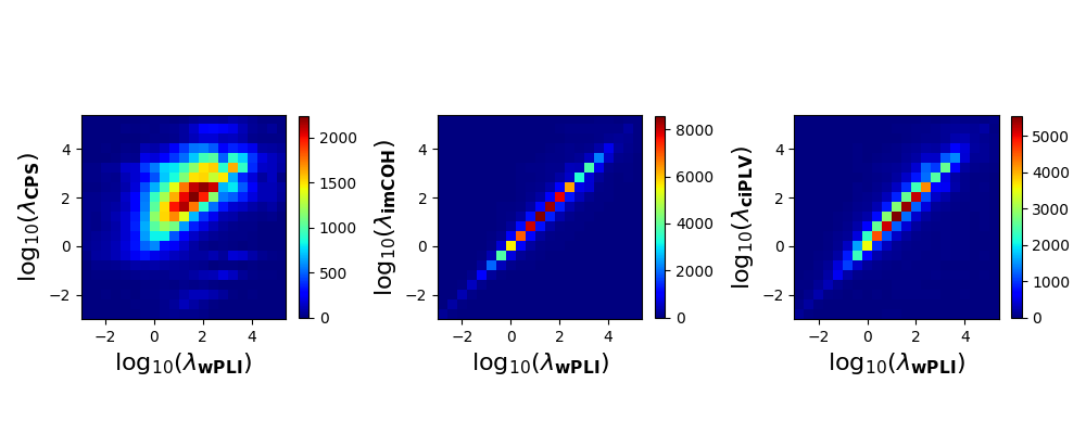
2D histogram showing the relationship between the optimal regularization parameters for different connectivity metrics. In each panel the x-axis shows the value of the optimal parameter for wPLI in logarithmic scale, while the y-axis refers to CPS, imCOH and ciPLV, respectively. Notice the different scale for the colorbar in each panel.
params = {'legend.fontsize': 14,
          'lines.linewidth': 3,
          'figure.figsize': (10, 4),
          'axes.labelsize': 16,
          'axes.titlesize': 18,
          'xtick.labelsize': 10,
          'ytick.labelsize': 10}
pylab.rcParams.update(params)

lam_cps = tested_par[np.argmax(-opt_par['conn'][:, :, :, :, :, :, 0, :],
                     axis=-1)]*opt_par['tc'][:, :, :, :, :, :, 0]
lam_imcoh = tested_par[np.argmax(-opt_par['conn'][:, :, :, :, :, :, 1, :],
                       axis=-1)]*opt_par['tc'][:, :, :, :, :, :, 0]
lam_ciplv = tested_par[np.argmax(-opt_par['conn'][:, :, :, :, :, :, 2, :],
                       axis=-1)]*opt_par['tc'][:, :, :, :, :, :, 0]
lam_wpli = tested_par[np.argmax(-opt_par['conn'][:, :, :, :, :, :, 3, :],
                      axis=-1)]*opt_par['tc'][:, :, :, :, :, :, 0]

fig, ax = plt.subplots(1, 3, tight_layout=True)
shrink = 0.5
origin = 'lower'
cmap = 'jet'
hist, ybins, xbins = np.histogram2d(np.log10(np.reshape(lam_cps, (-1, ))),
                                    np.log10(np.reshape(lam_wpli, (-1, ))),
                                    bins=[np.arange(-3, 5.5, 0.4),
                                    np.arange(-3, 5.5, 0.4)])
im1 = ax[0].imshow(hist, extent=[xbins[0], xbins[-1],
                   ybins[0], ybins[-1]], cmap=cmap, origin=origin)
fig.colorbar(im1, ax=ax[0], location='right', shrink=shrink)
ax[0].set_xlabel(r'log$_{10}(\lambda_\mathbf{wPLI})$')
ax[0].set_ylabel(r'log$_{10}(\lambda_\mathbf{CPS})$')
ax[0].set_xticks([-2, 0, 2, 4])
ax[0].set_yticks([-2, 0, 2, 4])


hist, ybins, xbins = np.histogram2d(np.log10(np.reshape(lam_imcoh, (-1, ))),
                                    np.log10(np.reshape(lam_wpli, (-1, ))),
                                    bins=[np.arange(-3, 5.5, 0.4),
                                    np.arange(-3, 5.5, 0.4)])
im2 = ax[1].imshow(hist, extent=[xbins[0], xbins[-1],
                   ybins[0], ybins[-1]], cmap=cmap, origin=origin)
fig.colorbar(im2, ax=ax[1], location='right', shrink=shrink)
ax[1].set_xlabel(r'log$_{10}(\lambda_\mathbf{wPLI})$')
ax[1].set_ylabel(r'log$_{10}(\lambda_\mathbf{imCOH})$')
ax[1].set_xticks([-2, 0, 2, 4])
ax[1].set_yticks([-2, 0, 2, 4])

hist, ybins, xbins = np.histogram2d(np.log10(np.reshape(lam_ciplv, (-1, ))),
                                    np.log10(np.reshape(lam_wpli, (-1, ))),
                                    bins=[np.arange(-3, 5.5, 0.4),
                                    np.arange(-3, 5.5, 0.4)])
im3 = ax[2].imshow(hist, cmap=cmap, extent=[xbins[0],
                   xbins[-1], ybins[0], ybins[-1]], origin=origin)
ax[2].set_xlabel(r'log$_{10}(\lambda_\mathbf{wPLI})$')
ax[2].set_ylabel(r'log$_{10}(\lambda_\mathbf{ciPLV})$')
ax[2].set_xticks([-2, 0, 2, 4])
ax[2].set_yticks([-2, 0, 2, 4])
fig.colorbar(im3, ax=ax[2], location='right', shrink=shrink)
<matplotlib.colorbar.Colorbar object at 0x7ffa9e463690>
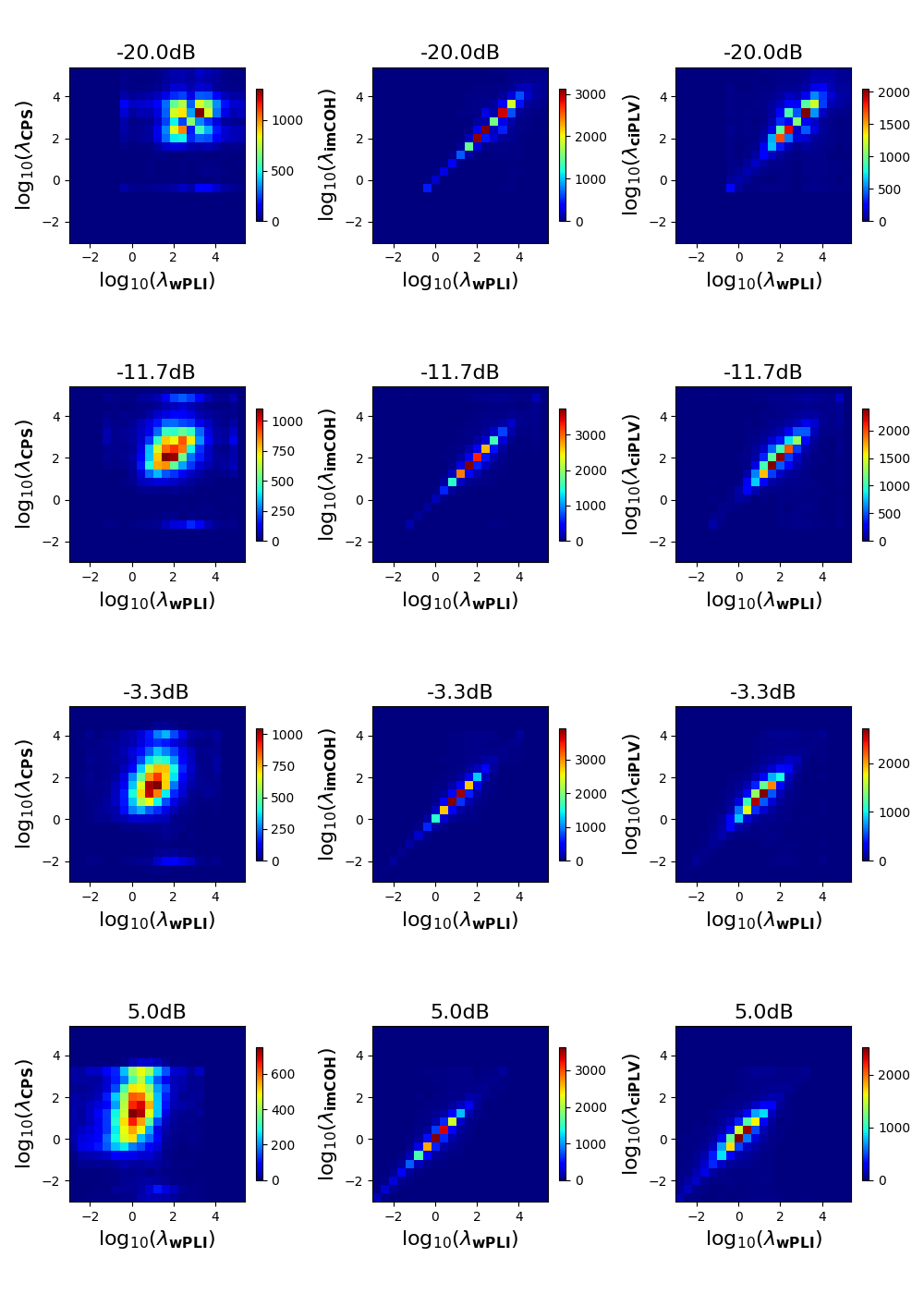
Impact of the measurement noise on the relationship between the optimal regularization parameters for different connectivity metrics. Each row refers to a different signal-to-noise ratio whose value is reported on top of the panels. Each column shows the 2D-histogram for a different pair of connectivity metrics, namely CPS vs wPLI (left column), imCOH vs wPLI (middle column), and ciPLV vs wPLI (right column)
params = {'legend.fontsize': 14,
          'lines.linewidth': 3,
          'figure.figsize': (10, 14),
          'axes.labelsize': 16,
          'axes.titlesize': 16,
          'xtick.labelsize': 10,
          'ytick.labelsize': 10}
pylab.rcParams.update(params)
fig, ax = plt.subplots(4, 3, tight_layout=True)

shrink = 0.47
origin = 'lower'
cmap = 'jet'

for i_snr in range(N_snr):
    lam_cps = tested_par[np.argmax(-opt_par['conn'][:, :, :, :, :, i_snr, 0,
                         :], axis=-1)]*opt_par['tc'][:, :, :, :, :, i_snr, 0]
    lam_imcoh = tested_par[np.argmax(-opt_par['conn'][:, :, :, :, :, i_snr, 1,
                           :], axis=-1)]*opt_par['tc'][:, :, :, :, :, i_snr, 0]
    lam_ciplv = tested_par[np.argmax(-opt_par['conn'][:, :, :, :, :, i_snr, 2,
                           :], axis=-1)]*opt_par['tc'][:, :, :, :, :, i_snr, 0]
    lam_wpli = tested_par[np.argmax(-opt_par['conn'][:, :, :, :, :, i_snr, 3,
                          :], axis=-1)]*opt_par['tc'][:, :, :, :, :, i_snr, 0]

    hist, ybins, xbins = np.histogram2d(np.log10(np.reshape(lam_cps, (-1, ))),
                                        np.log10(np.reshape(lam_wpli, (-1, ))),
                                        bins=[np.arange(-3, 5.5, 0.4),
                                        np.arange(-3, 5.5, 0.4)])
    im1 = ax[i_snr, 0].imshow(hist, extent=[xbins[0], xbins[-1],
                              ybins[0], ybins[-1]], cmap=cmap, origin=origin)
    fig.colorbar(im1, ax=ax[i_snr, 0], location='right', shrink=shrink)
    ax[i_snr, 0].set_xlabel(r'log$_{10}(\lambda_\mathbf{wPLI})$')
    ax[i_snr, 0].set_title(str(np.round(SNR_val[i_snr], decimals=1))+'dB')
    ax[i_snr, 0].set_xticks([-2, 0, 2, 4])
    ax[i_snr, 0].set_yticks([-2, 0, 2, 4])
    ax[i_snr, 0].set_ylabel(r'log$_{10}(\lambda_\mathbf{CPS})$')

    hist, ybins, xbins = np.histogram2d(np.log10(np.reshape(lam_imcoh, (-1, ))),
                                        np.log10(np.reshape(lam_wpli, (-1, ))),
                                        bins=[np.arange(-3, 5.5, 0.4),
                                        np.arange(-3, 5.5, 0.4)])
    im1 = ax[i_snr, 1].imshow(hist, extent=[xbins[0], xbins[-1],
                              ybins[0], ybins[-1]], cmap=cmap, origin=origin)
    fig.colorbar(im1, ax=ax[i_snr, 1], location='right', shrink=shrink)
    ax[i_snr, 1].set_xlabel(r'log$_{10}(\lambda_\mathbf{wPLI})$')
    ax[i_snr, 1].set_title(str(np.round(SNR_val[i_snr], decimals=1))+'dB')
    ax[i_snr, 1].set_xticks([-2, 0, 2, 4])
    ax[i_snr, 1].set_yticks([-2, 0, 2, 4])
    ax[i_snr, 1].set_ylabel(r'log$_{10}(\lambda_\mathbf{imCOH})$')

    hist, ybins, xbins = np.histogram2d(np.log10(np.reshape(lam_ciplv, (-1, ))),
                                        np.log10(np.reshape(lam_wpli, (-1, ))),
                                        bins=[np.arange(-3, 5.5, 0.4),
                                        np.arange(-3, 5.5, 0.4)])
    im1 = ax[i_snr, 2].imshow(hist, extent=[xbins[0], xbins[-1],
                              ybins[0], ybins[-1]], cmap=cmap, origin=origin)
    fig.colorbar(im1, ax=ax[i_snr, 2], location='right', shrink=shrink)
    ax[i_snr, 2].set_xlabel(r'log$_{10}(\lambda_\mathbf{wPLI})$')
    ax[i_snr, 2].set_title(str(np.round(SNR_val[i_snr], decimals=1))+'dB')
    ax[i_snr, 2].set_xticks([-2, 0, 2, 4])
    ax[i_snr, 2].set_yticks([-2, 0, 2, 4])
    ax[i_snr, 2].set_ylabel(r'log$_{10}(\lambda_\mathbf{ciPLV})$')
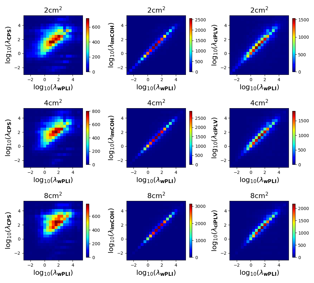
Impact of patch area
params = {'legend.fontsize': 14,
          'lines.linewidth': 3,
          'figure.figsize': (10, 9),
          'axes.labelsize': 16,
          'axes.titlesize': 16,
          'xtick.labelsize': 10,
          'ytick.labelsize': 10}

pylab.rcParams.update(params)
fig, ax = plt.subplots(3, 3, tight_layout=True)

shrink = 0.78
origin = 'lower'
cmap = 'jet'

for i_r in range(N_r):
    lam_cps = tested_par[np.argmax(-opt_par['conn'][:, :, i_r, :, :, :, 0,
                         :], axis=-1)]*opt_par['tc'][:, :, i_r, :, :, :, 0]
    lam_imcoh = tested_par[np.argmax(-opt_par['conn'][:, :, i_r, :, :, :, 1,
                           :], axis=-1)]*opt_par['tc'][:, :, i_r, :, :, :, 0]
    lam_ciplv = tested_par[np.argmax(-opt_par['conn'][:, :, i_r, :, :, :, 2,
                           :], axis=-1)]*opt_par['tc'][:, :, i_r, :, :, :, 0]
    lam_wpli = tested_par[np.argmax(-opt_par['conn'][:, :, i_r, :, :, :, 3,
                          :], axis=-1)]*opt_par['tc'][:, :, i_r, :, :, :, 0]

    hist, ybins, xbins = np.histogram2d(np.log10(np.reshape(lam_cps, (-1, ))),
                                        np.log10(np.reshape(lam_wpli, (-1, ))),
                                        bins=[np.arange(-3, 5.5, 0.4),
                                        np.arange(-3, 5.5, 0.4)])
    im1 = ax[i_r, 0].imshow(hist, extent=[xbins[0], xbins[-1],
                            ybins[0], ybins[-1]], cmap=cmap, origin=origin)
    fig.colorbar(im1, ax=ax[i_r, 0], location='right', shrink=shrink)
    ax[i_r, 0].set_xlabel(r'log$_{10}(\lambda_\mathbf{wPLI})$')
    ax[i_r, 0].set_title(str(np.round(area[i_r], decimals=1))+r'cm$^2$')
    ax[i_r, 0].set_xticks([-2, 0, 2, 4])
    ax[i_r, 0].set_yticks([-2, 0, 2, 4])
    ax[i_r, 0].set_ylabel(r'log$_{10}(\lambda_\mathbf{CPS})$')

    hist, ybins, xbins = np.histogram2d(np.log10(np.reshape(lam_imcoh, (-1, ))),
                                        np.log10(np.reshape(lam_wpli, (-1, ))),
                                        bins=[np.arange(-3, 5.5, 0.4),
                                        np.arange(-3, 5.5, 0.4)])
    im1 = ax[i_r, 1].imshow(hist, extent=[xbins[0], xbins[-1],
                            ybins[0], ybins[-1]], cmap=cmap, origin=origin)
    fig.colorbar(im1, ax=ax[i_r, 1], location='right', shrink=shrink)
    ax[i_r, 1].set_xlabel(r'log$_{10}(\lambda_\mathbf{wPLI})$')
    ax[i_r, 1].set_title(str(np.round(area[i_r], decimals=1))+r'cm$^2$')
    ax[i_r, 1].set_xticks([-2, 0, 2, 4])
    ax[i_r, 1].set_yticks([-2, 0, 2, 4])
    ax[i_r, 1].set_ylabel(r'log$_{10}(\lambda_\mathbf{imCOH})$')

    hist, ybins, xbins = np.histogram2d(np.log10(np.reshape(lam_ciplv, (-1, ))),
                                        np.log10(np.reshape(lam_wpli, (-1, ))),
                                        bins=[np.arange(-3, 5.5, 0.4),
                                        np.arange(-3, 5.5, 0.4)])
    im1 = ax[i_r, 2].imshow(hist, extent=[xbins[0], xbins[-1],
                            ybins[0], ybins[-1]], cmap=cmap, origin=origin)
    fig.colorbar(im1, ax=ax[i_r, 2], location='right', shrink=shrink)
    ax[i_r, 2].set_xlabel(r'log$_{10}(\lambda_\mathbf{wPLI})$')
    ax[i_r, 2].set_title(str(np.round(area[i_r], decimals=1))+r'cm$^2$')
    ax[i_r, 2].set_xticks([-2, 0, 2, 4])
    ax[i_r, 2].set_yticks([-2, 0, 2, 4])
    ax[i_r, 2].set_ylabel(r'log$_{10}(\lambda_\mathbf{ciPLV})$')
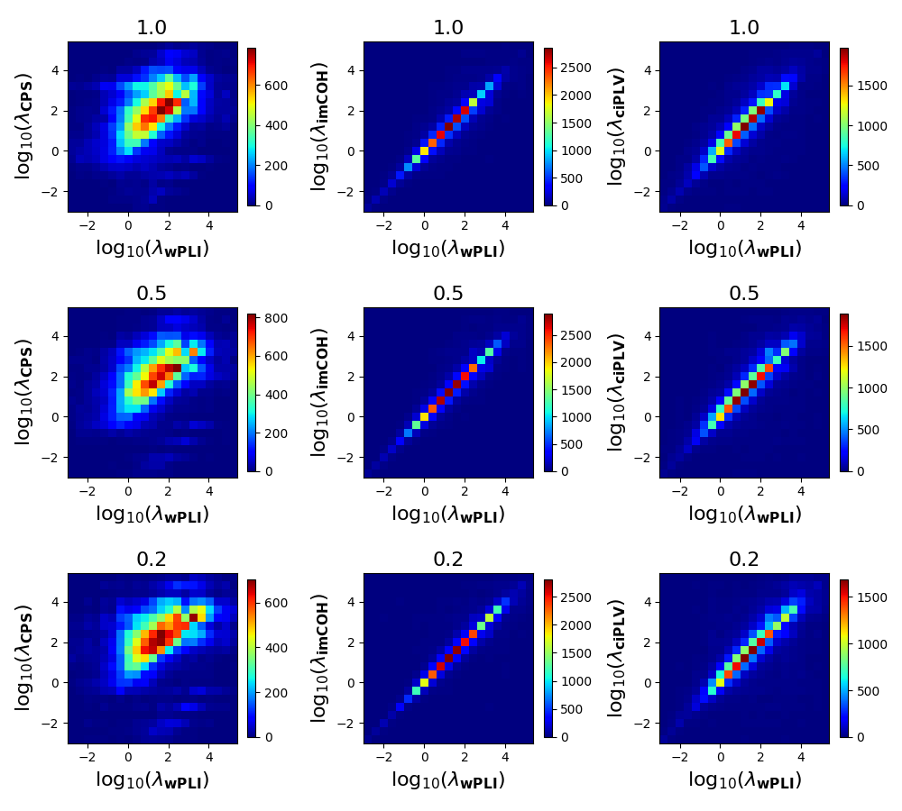
Impact of intra-patch coherence
params = {'legend.fontsize': 14,
          'lines.linewidth': 3,
          'figure.figsize': (10, 9),
          'axes.labelsize': 16,
          'axes.titlesize': 16,
          'xtick.labelsize': 10,
          'ytick.labelsize': 10}
pylab.rcParams.update(params)
fig, ax = plt.subplots(3, 3, tight_layout=True)

shrink = 0.78
origin = 'lower'
cmap = 'jet'

for i_c in range(N_c):
    lam_cps = tested_par[np.argmax(-opt_par['conn'][:, :, :, i_c, :, :, 0,
                         :], axis=-1)]*opt_par['tc'][:, :, :, i_c, :, :, 0]
    lam_imcoh = tested_par[np.argmax(-opt_par['conn'][:, :, :, i_c, :, :, 1,
                           :], axis=-1)]*opt_par['tc'][:, :, :, i_c, :, :, 0]
    lam_ciplv = tested_par[np.argmax(-opt_par['conn'][:, :, :, i_c, :, :, 2,
                           :], axis=-1)]*opt_par['tc'][:, :, :, i_c, :, :, 0]
    lam_wpli = tested_par[np.argmax(-opt_par['conn'][:, :, :, i_c, :, :, 3,
                          :], axis=-1)]*opt_par['tc'][:, :, :, i_c, :, :, 0]

    hist, ybins, xbins = np.histogram2d(np.log10(np.reshape(lam_cps, (-1, ))),
                                        np.log10(np.reshape(lam_wpli, (-1, ))),
                                        bins=[np.arange(-3, 5.5, 0.4),
                                        np.arange(-3, 5.5, 0.4)])
    im1 = ax[i_c, 0].imshow(hist, extent=[xbins[0], xbins[-1],
                            ybins[0], ybins[-1]], cmap=cmap, origin=origin)
    fig.colorbar(im1, ax=ax[i_c, 0], location='right', shrink=shrink)
    ax[i_c, 0].set_xlabel(r'log$_{10}(\lambda_\mathbf{wPLI})$')
    ax[i_c, 0].set_title(str(np.round(coh_levels[i_c], decimals=1)))
    ax[i_c, 0].set_xticks([-2, 0, 2, 4])
    ax[i_c, 0].set_yticks([-2, 0, 2, 4])
    ax[i_c, 0].set_ylabel(r'log$_{10}(\lambda_\mathbf{CPS})$')

    hist, ybins, xbins = np.histogram2d(np.log10(np.reshape(lam_imcoh, (-1, ))),
                                        np.log10(np.reshape(lam_wpli, (-1, ))),
                                        bins=[np.arange(-3, 5.5, 0.4),
                                        np.arange(-3, 5.5, 0.4)])
    im1 = ax[i_c, 1].imshow(hist, extent=[xbins[0], xbins[-1],
                            ybins[0], ybins[-1]], cmap=cmap, origin=origin)
    fig.colorbar(im1, ax=ax[i_c, 1], location='right', shrink=shrink)
    ax[i_c, 1].set_xlabel(r'log$_{10}(\lambda_\mathbf{wPLI})$')
    ax[i_c, 1].set_title(str(np.round(coh_levels[i_c], decimals=1)))
    ax[i_c, 1].set_xticks([-2, 0, 2, 4])
    ax[i_c, 1].set_yticks([-2, 0, 2, 4])
    ax[i_c, 1].set_ylabel(r'log$_{10}(\lambda_\mathbf{imCOH})$')

    hist, ybins, xbins = np.histogram2d(np.log10(np.reshape(lam_ciplv, (-1, ))),
                                        np.log10(np.reshape(lam_wpli, (-1, ))),
                                        bins=[np.arange(-3, 5.5, 0.4),
                                        np.arange(-3, 5.5, 0.4)])
    im1 = ax[i_c, 2].imshow(hist, extent=[xbins[0], xbins[-1],
                            ybins[0], ybins[-1]], cmap=cmap, origin=origin)
    fig.colorbar(im1, ax=ax[i_c, 2], location='right', shrink=shrink)
    ax[i_c, 2].set_xlabel(r'log$_{10}(\lambda_\mathbf{wPLI})$')
    ax[i_c, 2].set_title(str(np.round(coh_levels[i_c], decimals=1)))
    ax[i_c, 2].set_xticks([-2, 0, 2, 4])
    ax[i_c, 2].set_yticks([-2, 0, 2, 4])
    ax[i_c, 2].set_ylabel(r'log$_{10}(\lambda_\mathbf{ciPLV})$')
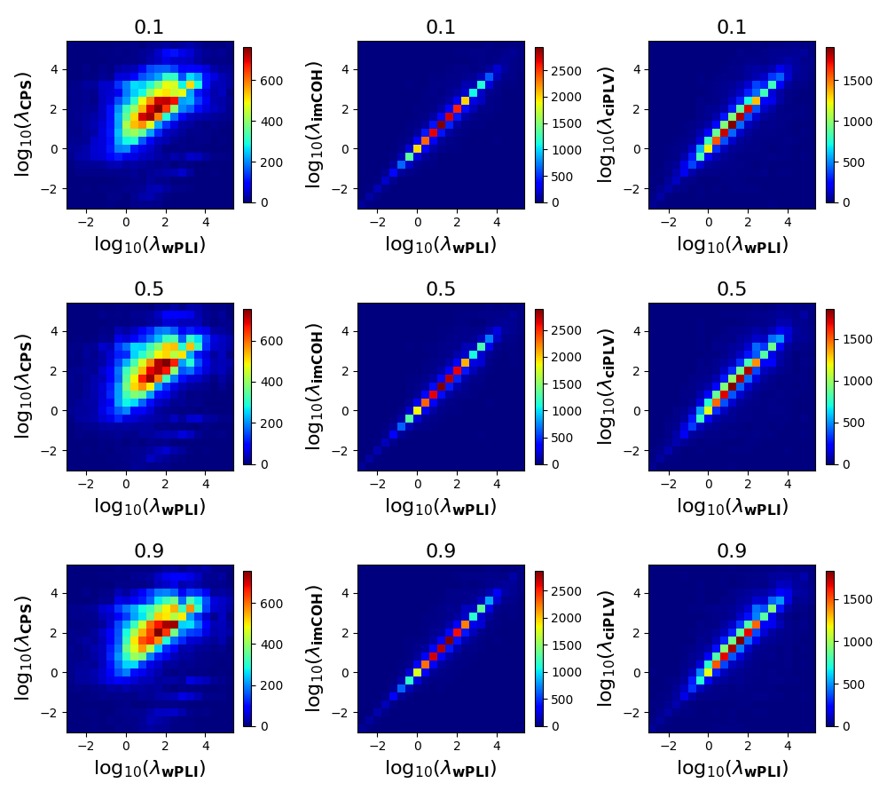
Impact of biological background noise.
params = {'legend.fontsize': 14,
          'lines.linewidth': 3,
          'figure.figsize': (10, 9),
          'axes.labelsize': 16,
          'axes.titlesize': 16,
          'xtick.labelsize': 10,
          'ytick.labelsize': 10}
pylab.rcParams.update(params)

fig, ax = plt.subplots(3, 3, tight_layout=True)

shrink = 0.78
origin = 'lower'
cmap = 'jet'

for i_gamma in range(N_gamma):
    lam_cps = tested_par[np.argmax(-opt_par['conn'][:, :, :, :, i_gamma, :,
                         0, :], axis=-1)]*opt_par['tc'][:, :, :, :, i_gamma,
                                                        :, 0]
    lam_imcoh = tested_par[np.argmax(-opt_par['conn'][:, :, :, :, i_gamma, :,
                           1, :], axis=-1)]*opt_par['tc'][:, :, :, :, i_gamma,
                                                          :, 0]
    lam_ciplv = tested_par[np.argmax(-opt_par['conn'][:, :, :, :, i_gamma, :,
                           2, :], axis=-1)]*opt_par['tc'][:, :, :, :, i_gamma,
                                                          :, 0]
    lam_wpli = tested_par[np.argmax(-opt_par['conn'][:, :, :, :, i_gamma, :,
                          3, :], axis=-1)]*opt_par['tc'][:, :, :, :, i_gamma,
                                                         :, 0]

    hist, ybins, xbins = np.histogram2d(np.log10(np.reshape(lam_cps, (-1, ))),
                                        np.log10(np.reshape(lam_wpli, (-1, ))),
                                        bins=[np.arange(-3, 5.5, 0.4),
                                        np.arange(-3, 5.5, 0.4)])
    im1 = ax[i_gamma, 0].imshow(hist, extent=[xbins[0], xbins[-1],
                                ybins[0], ybins[-1]], cmap=cmap, origin=origin)
    fig.colorbar(im1, ax=ax[i_gamma, 0], location='right', shrink=shrink)
    ax[i_gamma, 0].set_xlabel(r'log$_{10}(\lambda_\mathbf{wPLI})$')
    ax[i_gamma, 0].set_title(
        str(np.round(bg_noise_levels[i_gamma], decimals=1)))
    ax[i_gamma, 0].set_xticks([-2, 0, 2, 4])
    ax[i_gamma, 0].set_yticks([-2, 0, 2, 4])
    ax[i_gamma, 0].set_ylabel(r'log$_{10}(\lambda_\mathbf{CPS})$')

    hist, ybins, xbins = np.histogram2d(np.log10(np.reshape(lam_imcoh, (-1, ))),
                                        np.log10(np.reshape(lam_wpli, (-1, ))),
                                        bins=[np.arange(-3, 5.5, 0.4),
                                        np.arange(-3, 5.5, 0.4)])
    im1 = ax[i_gamma, 1].imshow(hist, extent=[xbins[0], xbins[-1],
                                ybins[0], ybins[-1]], cmap=cmap, origin=origin)
    fig.colorbar(im1, ax=ax[i_gamma, 1], location='right', shrink=shrink)
    ax[i_gamma, 1].set_xlabel(r'log$_{10}(\lambda_\mathbf{wPLI})$')
    ax[i_gamma, 1].set_title(
        str(np.round(bg_noise_levels[i_gamma], decimals=1)))
    ax[i_gamma, 1].set_xticks([-2, 0, 2, 4])
    ax[i_gamma, 1].set_yticks([-2, 0, 2, 4])
    ax[i_gamma, 1].set_ylabel(r'log$_{10}(\lambda_\mathbf{imCOH})$')

    hist, ybins, xbins = np.histogram2d(np.log10(np.reshape(lam_ciplv, (-1, ))),
                                        np.log10(np.reshape(lam_wpli, (-1, ))),
                                        bins=[np.arange(-3, 5.5, 0.4),
                                        np.arange(-3, 5.5, 0.4)])
    im1 = ax[i_gamma, 2].imshow(hist, extent=[xbins[0], xbins[-1],
                                ybins[0], ybins[-1]], cmap=cmap, origin=origin)
    fig.colorbar(im1, ax=ax[i_gamma, 2], location='right', shrink=shrink)
    ax[i_gamma, 2].set_xlabel(r'log$_{10}(\lambda_\mathbf{wPLI})$')
    ax[i_gamma, 2].set_title(
        str(np.round(bg_noise_levels[i_gamma], decimals=1)))
    ax[i_gamma, 2].set_xticks([-2, 0, 2, 4])
    ax[i_gamma, 2].set_yticks([-2, 0, 2, 4])
    ax[i_gamma, 2].set_ylabel(r'log$_{10}(\lambda_\mathbf{ciPLV})$')
Total running time of the script: ( 0 minutes 4.238 seconds)